Psy
Analysis
of Variance (ANOVA) is a hypothesis test that evaluates the significance
of mean differences.
Goal: Determine
whether the mean differences that are found in sample data are greater than can
be reasonably explained by chance alone. ANOVA can be used to evaluate
differences between two or more treatments (or populations).
How is ANOVA like the
t-test?
What advantage does
ANOVA have that t-tests do not?
A
typical situation in which ANOVA would be used--Three separate samples are
obtained to evaluate the mean differences among three populations (or
treatments) with unknown means.
We
want to decide between the following 2 hypotheses:
![]()
H1:
At least one population mean is different from another.

What is a factor?
Note: the scores are
not all the same—they are variable. We want to measure the amount of
variability (the size of the differences) and to explain where it comes from.
II. Logic
The analysis of
variance divides total variability into two parts—between treatments variance
and within-treatments variance.
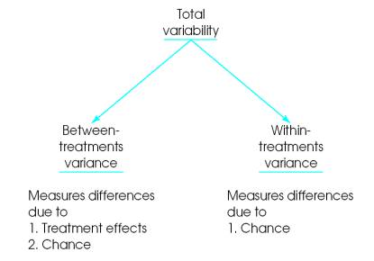

Finally, the two
variances are compared in an F-ratio to determine whether the mean
differences (MSbetween) are significantly bigger than chance (MSwithin).
When the treatment
has no effect, the F-ratio
should have a value around ____.
When the treatment
does have an effect, we should obtain an F-ratio noticeably larger than ___.
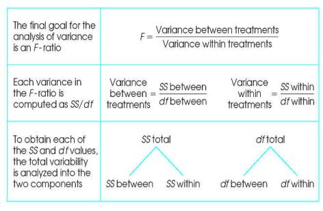
III.
Notation and Formulas

k
= # of treatments (# of levels of the factor)
n = # of scores in
each treatment. For example, n3 is the number of scores in treatment
3.
N = total # of scores
in the entire study. When n is the same for all treatments, then N = kn. For the
sample data, there are n = 5 scores in each of the k = 3 treatments, so N = 3
(5) = 15.
T = total of the
scores (ΣX) for each treatment condition. For example, the total for the
third treatment is T3 = 5.
G = the sum of all
the scores in the study (the grand total). Compute G by adding up all N scores
or adding up all of the treatment totals: G = ΣT.
Some important
preliminary calculations: (1) ΣX for each treatment condition, (2) ΣX2 for
each treatment and the entire data set, (3)
SS for each treatment condition and (4) n for each treatment condition.

IV. The
Distribution of F-ratios
When Ho is true, we
expect the value of F to be around 1.00. What do we mean by “around 1.00”? We
need to look at all the possible F values—the distribution of F-ratios.
1.
F-ratios are computed from two variances and variances must always be
positive, so F values will always be positive.
2.
When Ho is true, the numerator and denominator are measuring the same
variance so the ratio should be near 1. So notice that the distribution of
F-ratios piles up at 1.00.
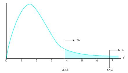
The
distribution of F-ratios
with df = 2,12. Of all the values in
the distribution, only 5% are larger than F = 3.88, and only 1% are larger
than F
= 6.93.
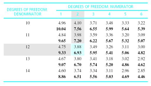
In ANOVA, what exactly does a significant result mean?
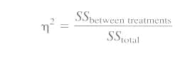
In order to indicate the how large the effect actually is, it is recommended that a measure of effect size be provided in addition to the measure of significance.
We want to determine how much of the differences between scores is accounted for by the differences between treatments. Remember r2? It measures the proportion of the total variability that is accounted for by the differences between treatments. When computed for ANOVA, r2 is usually referred to as eta squared.
VI. Post Hoc Tests
Post hoc tests (posttests) are additional hypothesis tests that are done after the overall analysis of variance to determine exactly which mean differences are significant and which are not.
Post hoc tests are done after the overall ANOVA when:
You reject the Ho for the overall analysis and
There are three or more treatment conditions
Post hoc tests enable you to go back to the means and compare the means two at a time--pairwise comparisons
Type I errors and multiple hypothesis tests--
testwise alpha--each hypothesis test has a risk of type one error
associated with it
As you do more and more separate tests, the risk of a Type I
error accumulates and is called experimentwise alpha
Approx. experimentwise alpha=(c) (testwise alpha)
So we must be concerned with experimentwise alpha whenever we
conduct post hoc tests. Statisticians have determined several methods for
controlling experimentwise alpha.
Which method of control we use depends on the type of comparison: planned or
unplanned
A few planned comparisons can be conducted with the standard alpha level without worrying about an inflated experimentwise alpha. If many planned comparisons, use the Dunn test--divide the standard alpha equally by the number of comparisons.
There are many correction methods for unplanned comparisons--We will cover Tukey's HSD.